Explore and Optimize Multi-Physics Design Spaces with AI Physics

AI Physics introduces Explorations — a new feature for design space exploration and optimization using trained surrogate models. Build multi-physics systems by wiring together geometry, models, and scripts on a visual canvas, then run sweeps or optimizations across hundreds of design variants.

What makes this powerful: you can combine multiple physics disciplines in a single study. Run CFD and FEA surrogate models together — for example, optimizing an impeller's geometry for both aerodynamic performance and structural stress simultaneously, in a fraction of the time required for traditional simulations.

Release Highlights

What is it?

Explorations bring three capabilities together:

• System Builder — A visual canvas where you design multi-physics pipelines by connecting blocks: Input (design variables), Geometry (parametric shapes), Model (surrogate models), Script (custom logic to bridge physics), and Output. This is the core of the feature — it lets you compose arbitrarily complex systems, including multi-physics setups that chain CFD and FEA models with scripted data transformations between them as needed.

• Sweep (DOE) — Sample the design space using strategies like Latin hypercube sampling to efficiently cover high-dimensional parameter spaces. Auto-calibrated parallel execution probes for the fastest throughput on your machine.

• Optimize — Run single or multi-objective optimization to converge on optimal designs, with NSGA-II or weighted search methods.

Why does it matter?

Previously, multi-physics optimization with surrogate models required writing custom code and manually orchestrating data flow between models from different disciplines. There was no supported way to combine, say, a CFD surrogate and an FEA surrogate in a single optimization loop.

Explorations eliminates that barrier. The System Builder lets you visually wire together models from different physics domains, add script nodes to transform data between them (e.g., mapping CFD pressure outputs to FEA boundary conditions), and treat the entire pipeline as a single system to sweep or optimize. Engineers who build simulations can now build optimization runs the same way — by connecting blocks on a canvas.

The speed advantage compounds with multi-physics. Instead of running two full solvers per design variant, surrogate inference evaluates each case in seconds per model. A study that would be computationally infeasible with traditional simulation becomes a 10-minute run.

How is it used?

Any user with trained surrogate models in AI Physics can create an Exploration. Once the surrogate models are configured into a System, create a new Run in the following three steps:

• Configure - Select which design variables to vary, set their min/max bounds, and choose which outputs to record. The system automatically discovers variables from your Input node and traces which models and geometry blocks they feed into.

• Explore - Choose between Sweep (DOE) or Optimize. For sweeps, pick a sampling strategy and sample count. For optimization, define objectives (maximize, minimize) and select an algorithm. Set the execution plan — Auto mode probes for the optimal number of parallel workers.

• Execute - Monitor progress as cases run, then review results. Sweep results include 2D scatter plots, 3D visualizations, heat maps, and a Trade Space view. Optimization results show the Pareto front, driver analysis, constraint satisfaction, and a gallery of the best-design geometries rendered as images — so you can visually compare the shapes the optimizer discovered.

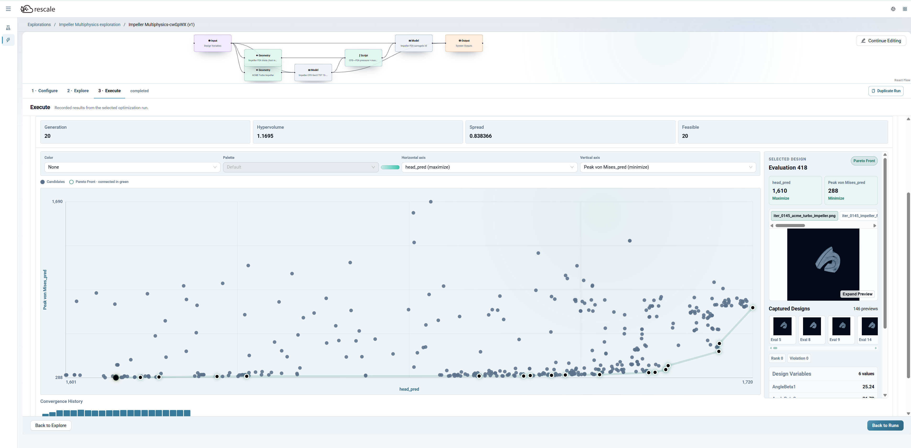
Optimization results showing the Pareto front and best-design geometries

Getting Started

1. Navigate to Explorations from the left sidebar in AI Physics Training and click Start Exploration.

2. Give your exploration a name and description, then Add Models — select the trained surrogate models you want to use. Each model lists its Inference Bundles and Candidates.

3. Click Build System to open the System Builder canvas. Wire together your pipeline: drag blocks from the left panel (Input, Output, Geometry, Model, Script, Math, Constraint) and connect them. For multi-physics, add multiple Geometry and Model blocks and use a Script node to bridge data between disciplines.

4. Return to your Exploration home page and click New Run.

5. In Configure, toggle which variables to vary, set bounds, and choose reference values.

6. In Explore, select Sweep (DOE) or Optimize, configure sampling or objectives, and launch.

7. In Execute, review results — use the Overview, Drivers, Constraints, and Artifacts tabs to analyze outcomes. Export to CSV or duplicate the run to iterate.

Start with a sweep to map the design space before running an optimization. The sweep helps you set meaningful bounds and objectives.

For more on building surrogate models, see the AI Physics documentation.